Tian Correction

Example Workflow

Load the Data

For fast reactions, e.g., reactions occurring during the first minutes of cement hydration, the thermal inertia of the calorimeter significantly broadens the heat flow signal. If the characteristic time constants are determined experimentally, a Tian correction can be applied to the heat flow data.

First we load the data.

from pathlib import Path

import matplotlib.pyplot as plt

from calocem import Measurement, ProcessingParameters

datapath = Path(__file__).parent / "calo_data"

# load experimental data
tam = Measurement(
    folder=datapath,
    regex=r".*file1.csv",
    show_info=True,
    auto_clean=False,
    cold_start=True,
)

In the next step, we need to define a few parameters which are necessary for the Tian correction. Therefore we create a ProcessingParameters object which we call processparams in this case. The processparams object has a number of attributes which we can define. First, we define two time constants tau1 and tau2. The numeric value needs to be determined experimentally.

# Set Processing Parameters
processparams = ProcessingParameters()
processparams.time_constants.tau1 = 240
processparams.time_constants.tau2 = 80
processparams.median_filter.apply = True
processparams.median_filter.size = 15
processparams.spline_interpolation.apply = True
processparams.spline_interpolation.smoothing_1st_deriv = 1e-10
processparams.spline_interpolation.smoothing_2nd_deriv = 1e-10

Next we apply the Tian correction by calling the method apply_tian_correction(). We pass the processparams object defined above to the method.

# apply tian correction
tam.apply_tian_correction(
    processparams=processparams,
)

Finally, we can get the Pandas dataframe containing the calorimetric data by calling get_data(). Using the df DataFrame we can plot the calorimetry data using well-known Matplotlib methods.

df = tam.get_data()

# plot corrected and uncorrected data
fig, ax = plt.subplots()
ax.plot(
    df["time_s"] / 60,
    df["normalized_heat_flow_w_g"],
    linestyle="--",
    label="sample"
    )
ax.plot(
    df["time_s"] / 60,
    df["normalized_heat_flow_w_g_tian"],
    color=ax.get_lines()[-1].get_color(),
    label="Tian corrected"
    )
ax.set_xlim(0, 15)
ax.set_xlabel("Time (min)")
ax.set_ylabel("Normalized Heat Flow (W/g)")
ax.legend()
plt.show()

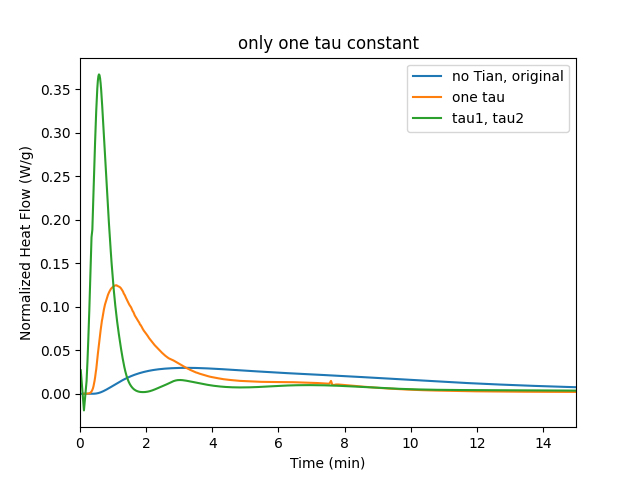
One or Two Tau Values

If only one Tau value is defined, the correction algorithm will only consider this \(\tau\) value and the data will be corrected according to

\[ P(t) = \varepsilon \left[ U(t) + \tau \frac{dU(t)}{dt} \right] \]

If two values for \(\tau\) are provided, the data will be corrected considering both values.

\[ P(t) = \varepsilon \left[ U(t) + (\tau_1+\tau_2) \frac{dU(t)}{dt} + \tau_1\tau_2 \frac{d^2U}{dt^2} \right] \]

The actual implementation of the correction algorithm is not based on the voltage \(U\) but on the heat flow. In most cases, the exported data does not contain the raw voltage data but the heat flow data which has been obtained in the instrument software with the experimentally determined value for \(\varepsilon\).

Therefore, the second equation reads like

\[ \dot{Q}_{Tian}(t) = \dot{Q}(t) + (\tau_1+\tau_2) \frac{\dot{Q}}{dt} + \tau_1\tau_2 \frac{d^2\dot{Q}}{dt^2} \]

In practical terms, if only the attribute tau1 is set, only the first derivative of the heat flow will be considered.

# Set Processing Parameters
processparams = ProcessingParameters()
processparams.time_constants.tau1 = 300

The difference between having one or two tau constants can be seen in the following plot. In general, having two tau constants renders the signal even more narrow.

Smoothing the Data

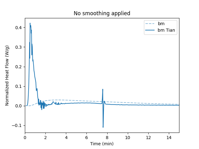
No smoothing

It is important to smoothen the data. Otherwise, small noise in the raw heat flow data will lead to significant noise especially in the second derivative. By default the smoothing is not applied. Here, we explicitly set the attributes to False and repeat the analysis as shown above. The results demonstrates the noise in the data which originates from tiny fluctuations which result in significant noise in the second derivative.

# Set Processing Parameters
processparams.median_filter.apply = False
processparams.spline_interpolation.apply = False

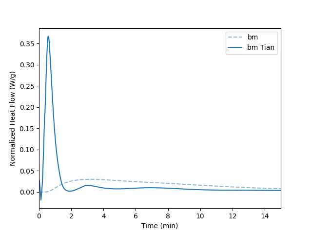
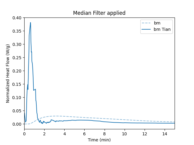
Only Median Filter

Here is the result of only applying a median filter with a size of 15.

# Set Processing Parameters
processparams.median_filter.apply = True
processparams.median_filter.size = 15
processparams.spline_interpolation.apply = False

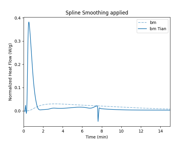
Only Spline Smoothing

Here is the result of only applying a Univariate Spline with smoothing of 1e-10 for both the first and the second derivative. The combination of a median filter and spline smoothing reliably delivers smooth data without introducing artifacts or significant line broadening.

# Set Processing Parameters
processparams.median_filter.apply = False
processparams.spline_interpolation.apply = True
processparams.spline_interpolation.smoothing_1st_deriv = 1e-10
processparams.spline_interpolation.smoothing_2nd_deriv = 1e-10